Detecting anomalies at all is hard; it’s even harder when you don’t know what’s an ‘anomaly.’ So what is anomaly detection in manufacturing?
Anomaly detection in manufacturing is the process of identifying data points that lie outside of the ‘norm’ and are rare in occurrence. In the manufacturing industry, anomalies usually are, or strongly indicate, defects in production that will later result in a loss to the manufacturer.
Traditional anomaly detection techniques such as clustering techniques, isolation decision trees, and other statistical approaches (intro-level overview found here) rely heavily on two assumptions:
- All data points are independent.
- What constitutes an anomaly is in unknown, and so it is possible to label abnormalities.
But what happens when this is no longer true?

What happens when data points are not independent?
Time invariance means that whether we apply an input to the system now or T seconds from now, the output will be identical except for a time delay of T seconds. — Wikipedia
When data points are not independent, a data point is both ‘normal’ AND an ‘anomaly,’ and it is the previous data that serves as the differentiation. This dependency makes the task of classifying anomalies magnitudes of order harder. When data points are not independent, algorithms derived from linear algebra will no longer apply (not to mentioned convergence is far from guaranteed), ruling out the use of most common approaches.
In machine learning, this issue presents even a bigger problem. Time dependency in data that is not inherently Time-Series (i.e., a series of values originating from a single process over time) introduces issues generally associated with data-drift, which is a significant problem for production-level models. ML-Ops — a fast-growing new industry — is responsible for detecting and alerting users of data-drift, the standard response being stopping the model, and replacing it. Ironically, this behavior is the norm rather than the anomaly when dealing with time-dependent anomaly detection.

What happens when the ‘anomaly’ class isn’t well defined?
In a supervised learning environment, we could easily split our data into straight forward classes of ‘normal’ and ‘anomaly.’ Indeed, the dataset will be strongly imbalanced (in some extreme cases, >97% will be ‘normal’). However, still, traditional techniques will be able to provide a significant boost (or ‘lift’) when compared to random selection.
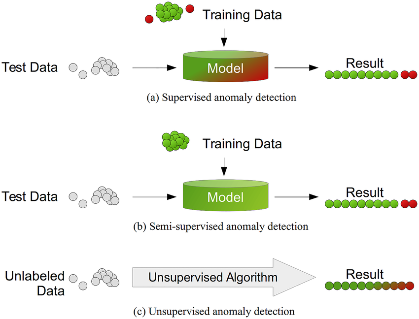
If, however, we cannot clearly define or recognize an anomaly in the training phase, we find ourselves in an unsupervised learning environment. Unsupervised learning lends to clustering techniques (such as KNN or DBScan). In essence, clustering techniques estimate one or more centers of mass around which many data points group by finding the point at which the overall sum of distances reaches a minimum. While many different distance metrics can prove useful, all work similarly. Any data point whose distance from all centers of mass is above some threshold is considered an anomaly (or outlier).
The effect of unsupervised learning on performance introduces a performance trade-off. The user may choose a threshold to satisfy either false positive or false negative — but never both.

Combining the two effects
When data is both time-variant and not labeled, we may categorize the problem as ‘time-dependent unsupervised anomaly detection.’ In simple terms, an unsupervised classification problem where the outcome depends on previous states. In terms of technological challenge, the difficulties presented by either issue is compounded by the other, negating the efficacy of traditional approaches for unsupervised classification and limiting the ability of time-series approaches.
The intersection of the solution space after ruling out unsupervised classification techniques and time-series techniques leaves an empty set, or a lot of room for innovation for the ‘glass half full’ reader.
A novel approach to anomaly detection in manufacturing
The approach proposed here is an iterative — Reinforcement Learning type — architecture that leverages time dependency to improve the overall performance continuously.
step #1
— the network at time T classifies a data snapshot at time T
Encoding (a good overview of sequential encoder-decoder here)
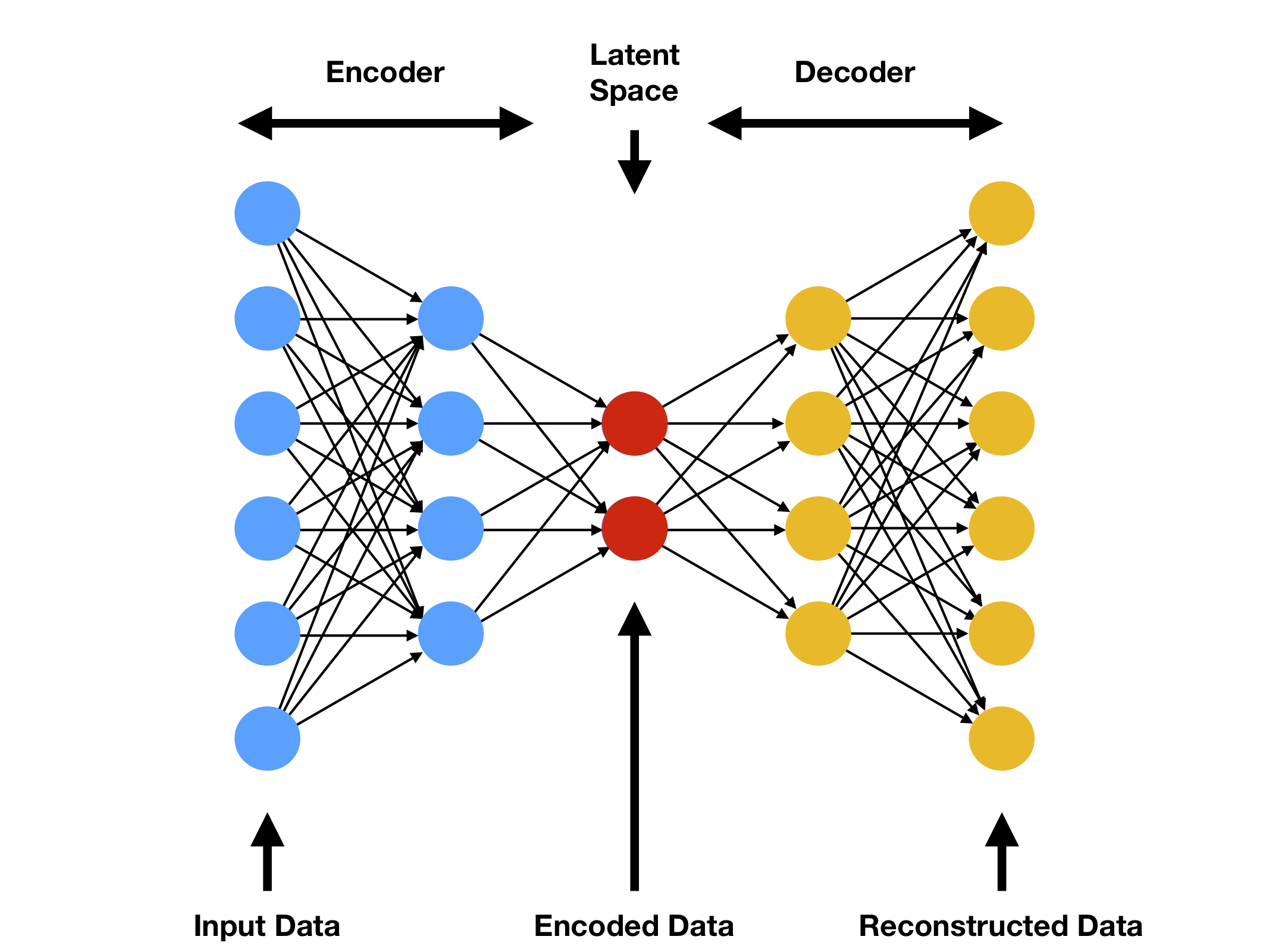
An encoder is a network taking in input data and transforming it to a new data set represented in a different feature-space (latent space) — usually smaller than the original feature-space, yet encapsulating all the information of the initial input.
In this approach, we manipulate the encoder such that the data represented in the encoder space provides better separation between the ‘normal’ and ‘anomaly’ classes. The smart construction of the encoding network performs this manipulation based on metrics of distance at the encoded space.
step #2 — a posterior cost function estimates the performance at time T
In a supervised learning environment defining the cost function for performance, estimation would be as straightforward as counting the number of errors (both false positive and false negative). In unsupervised learning, errors are unknown, requiring consideration of various techniques for performance evaluation.
One possible technique is to measure the degree of separation between clusters (or classes), the reasoning being that if the clusters are well separated, then the classification accuracy will be acceptable. There are a few caveats to this approach:
- A good separation of clusters doesn’t necessarily ensure that the clusters are ‘normal’ and ‘anomaly.’
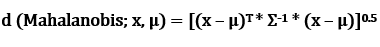
- Distance metric — Euclidean distance between two clusters (or their center of mass) is the ‘ruler distance’ and assumes variable independence (in mathematical terms, there’s a right angle between axes). However, if variables are dependent, a more suitable metric would be the Mahalanobis distance. For uncorrelated variables, the Euclidean distance equals the MD.
The Mahalanobis distance is a measure of the distance between a point P and a distribution D, introduced by P. C. Mahalanobis in 1936.[1] It is a multi-dimensional generalization of the idea of measuring how many standard deviations away — Wikipedia
Another approach would be to use the manufacturer (or user) as an annotation service down the line (or post-decision). Assuming the latency is tolerable, the classified results will continue through the manufacturer’s production line, where errors eventually surface. This approach will only work in scenarios where the convergence time and cost are tolerable by the end-user.
Another approach is to use the decoder half of the autoencoder network. The decoder performs the complementary action to the encoder and reverts the transformation into the latent space representation. The decoder can take the classified points, transform them into the original feature space; those points who return ‘too different’ from their original place are considered anomalies. Comparing the decoder labeled anomalies with the classifier labeled anomalies can provide a useful estimator of performance.
step #3 — the optimizing strategy optimizes the encoder construction parameters
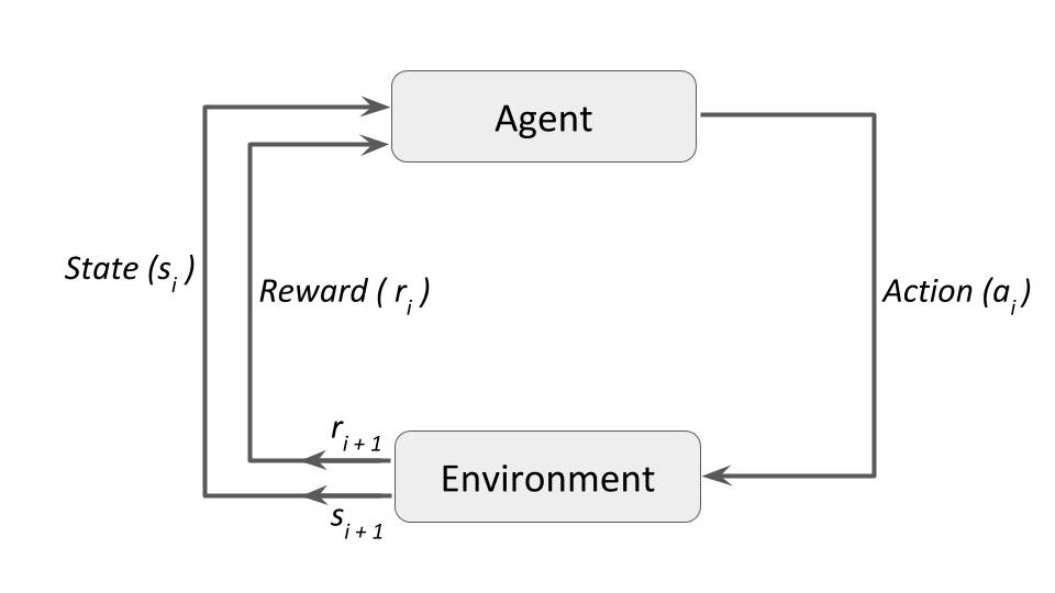
In reinforcement learning (RL — for a good overview, click here), the agent continuously updates the action or strategy acting on the environment to improve performance through higher rewards.
Similarly, using the cost function defined in step #3, the optimizing agent can explore various encoding strategies to reduce the overall cost. In the proposed approach, the encoder changes the encoder architecture based on the optimizing agent’s recommended ‘strategy.’
A bonus to this approach is introducing a de facto performance tracker; the automated update strategy to the encoder functions similarly to a PLL (Phase Locked Loop). Changes in data degrade performance; this is sensed by the optimizer, who updates the encoder to restore overall accuracy to an optimal level.
step #4 — the network at time T+1 classifies a data snapshot at time T+1
rinse & repeat.

Results
We consider the following scenario to evaluate performance:
- The manufacturer provided real-world data observations from a manufacturing line every 1 second
- The error rate (=anomaly rate) in the data was ~1% on average
- The manufacturer did not provide labels for anomalies
- The manufacturer provided a reading of the error rate based on an undisclosed method
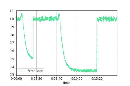
The algorithm reduces the overall error rate baseline of 1% to ~0.3% with a convergence time of ~2 minutes.
At around the 3-minute mark, the operator stopped the algorithm, and the error rate returned to 1%.
At around the 7-minute mark, the algorithm is reintroduced and let run until convergence at ~0.3% error rate — 3X better than before.
Summary of Anomaly Detection in Manufacturing
Anomaly detection is one of the more challenging tasks in data science today, and even more challenging when what constitutes an anomaly is unknown.
Present here is the high-level outline of Vanti’s proprietary approach along benchmark results achieving a 3X boost in anomaly detection in too harsh conditions.